This tutorial aims to explore various types of tools of visualizing the process data.
Before diving into the main text, I found one trick to
git pull one repo but ignore the local changes is:
git clean -f
git pull
Load Packages
A little about the toy data
A dataset containing the response processes and binary response outcomes of 16763 respondents. seqs is an object of class “proc” containing the action sequences and the time sequences of the respondents and responses is binary responses of 16763 respondents. The order of the respondents matches that in seqsß.
str(cc_data, max.level = 2)
List of 2
 $ seqs     :List of 2
  ..$ action_seqs:List of 16763
  ..$ time_seqs  :List of 16763
  ..- attr(*, "class")= chr "proc"
 $ responses: Named int [1:16763] 0 1 1 1 0 0 0 0 0 0 ...
..- attr(*, "names")= chr [1:16763] "ARE000000200039" "ARE000000200051" "ARE000000300079" "ARE000000400093" ...head(cc_data$seqs$action_seqs, n = 3)
$ARE000000200039
 [1] "start"    "0_0_0"    "1_2_-2"   "2_2_2"    "2_2_2"    "2_2_2"
 [7] "2_2_2"    "2_2_2"    "2_2_-2"   "2_2_-2"   "2_-2_-2"  "-2_-2_-2"
[13] "-2_-2_-2" "-2_-2_-2" "-2_-2_-2" "-2_-2_-2" "-2_-2_0"  "-2_-2_0"
[19] "-2_-2_0"  "-2_0_1"   "-2_0_1"   "-2_0_1"   "-2_0_1"   "-2_0_1"
[25] "0_0_1"    "0_0_1"    "0_0_1"    "0_0_1"    "0_0_1"    "0_0_1"
[31] "0_0_1"    "0_0_1"    "0_0_1"    "0_0_1"    "0_0_1"    "end"

$ARE000000200051
 [1] "start"    "reset"    "-1_0_0"   "-1_-1_0"  "-1_-1_-1" "-1_0_0"
 [7] "-1_0_0"   "reset"    "2_0_0"    "reset"    "0_2_0"    "reset"
[13] "0_0_2"    "reset"    "0_1_0"    "reset"    "0_-1_0"   "reset"
[19] "-1_0_0"   "reset"    "end"

$ARE000000300079
[1] "start" "1_1_1" "reset" "0_0_1" "reset" "0_1_0" "reset" "1_0_0"
[9] "end"
Data Transformation
## actions
dt1 <- cc_data$seqs$action_seqs[1:30]
## time stamps
dt2 <- cc_data$seqs$time_seqs[1:30]
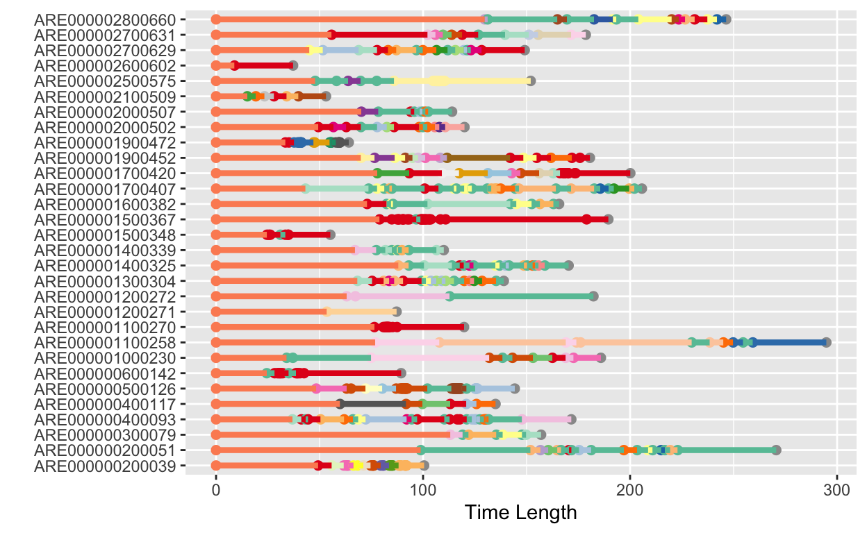
## x轴为时间轴,y轴为不同的observations
dt1_long <- mapply(function(x, y) data.frame(ID = y, action = x) , dt1, names(dt1), SIMPLIFY = FALSE)
dt1_long <- Reduce(rbind, dt1_long)
dt2_long <- mapply(function(x, y) data.frame(ID = y, time = x) , dt2, names(dt2), SIMPLIFY = FALSE)
dt2_long <- Reduce(rbind, dt2_long)
dt_full <- cbind(dt1_long, time = dt2_long[,2]) %>%
group_by(ID) %>%
mutate(time_upper = lead(time)) %>%
ungroup() %>%
mutate(time_upper = ifelse(is.na(time_upper), time, time_upper), action = as.factor(action))
head(dt_full)
# A tibble: 6 × 4
  ID              action  time time_upper
  <chr>           <fct>  <dbl>      <dbl>
1 ARE000000200039 start    0         49.3
2 ARE000000200039 0_0_0   49.3       55.9
3 ARE000000200039 1_2_-2  55.9       61.7
4 ARE000000200039 2_2_2   61.7       62.6
5 ARE000000200039 2_2_2   62.6       63.2
6 ARE000000200039 2_2_2   63.2       63.5
Data Visualization
set.seed(1234)
n <- 30 # 30 colors
qual_col_pals = brewer.pal.info[brewer.pal.info$category == 'qual',]
col_vector = unlist(mapply(brewer.pal, qual_col_pals$maxcolors, rownames(qual_col_pals)))
line_color = sample(col_vector, n)

ggplot(aes(x = time, y = ID, col = action), data = dt_full) +
  geom_point(size = 2)+
  geom_linerange(aes(xmin = time, xmax= time_upper), linetype = 1, size = 1.5)+
  scale_color_manual(values = col_vector, name = "") +
  labs(y = "", x = "Time Length") +
  theme(legend.position="")